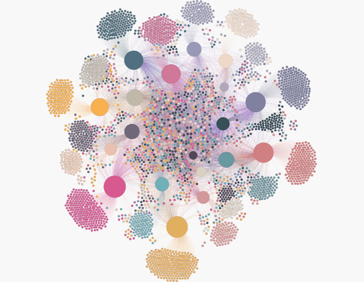
"Weil alles mit (fast) allem
(zumindest ein wenig) zusammen hängt."
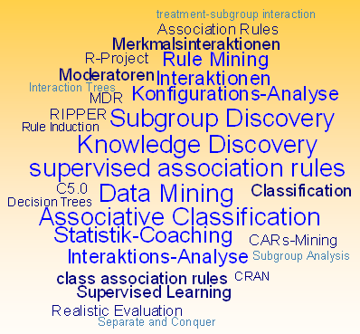
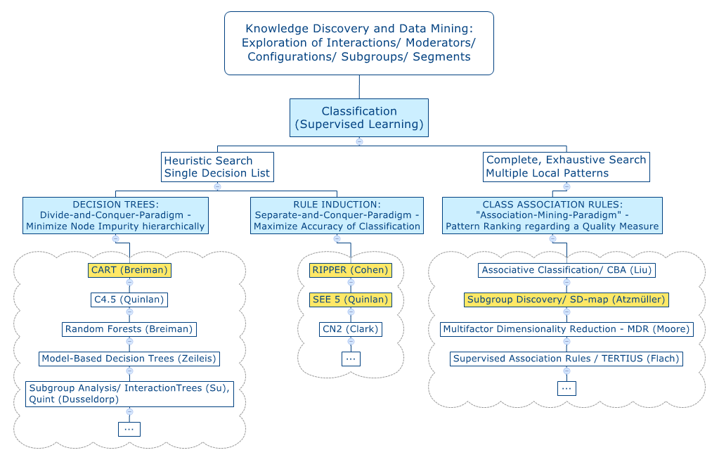
CARs - Mining:
Data Mining
von Merkmalsinteraktionen
|
"Weil alles mit (fast) allem (zumindest ein wenig) zusammen hängt." |
|
|
|
CARs - Mining: Data Mining
von Merkmalsinteraktionen
|
| 1. Ausgangssituation und Problemstellung |

| Wenn zumindest ein Teil der hier aufgeführten Aussagen auf Ihre Problemstellung zutrifft, dann sind Sie auf dieser Seite goldrichtig. |
|
|
| 2. Statistik - Coaching |
 |
 |
| Nummer zur Navigation | Kapitel | Inhalte | Zielgruppe |
| 1 | Ausgangssituation
und Problemstellung |
Welches Auswertungsverfahren für welche Daten? | speziell für Anfänger |
| 2 | Statistik-Coaching | Anleitung für selbständige Auswertungen, Beratungsbedarf, Kontaktaufnahme, Navigation und Inhaltsverzeichnis | |
| 3 | Illustrierendes
Beispiel zum CARs - Mining |
Kleine fiktive Daten-Datei | speziell für Anfänger |
| 4 | Beispiel
2: Komplexe 3-Weg Interaktion |
Im
Vergleich: CARs - Mining, CART- Entscheidungsbaum, Rule Induction mit SEE5 und RIPPER |
|
| 5 | Beispiel
3: Haupteffekte reichen aus |
Im
Vergleich: CARs - Mining, CART- Entscheidungsbaum, Rule Induction mit SEE5 und RIPPER, logistische Regression, lineare Diskriminanzanalyse |
|
| 6 | Hinweise
und Tipps zur Durchführung von CARs - Mining |
Diskretisierung der unabhängigen Merkmale, optionale Diskretisierung der Zielgröße, Imputation von fehlenden Werten, Qualitätsmaße im CARs - Mining, Suchalgorithmen, Visualisierung der Ergebnisse, "Wer nur einen Hammer als Werkzeug hat ..." , CARs - Mining und verwandte Verfahren, Fazit | |
| 7 | Freeware
zum CARs - Mining |
Auflistung mit Link | |
| 8 | Kleine Einführung in die Nutzung der Software R-Project von CRAN | Hinweise zur Installation und zum Arbeiten mit der Freeware R-Project | speziell für Anfänger |
| 9 | CARs - Mining mit WEKA | Anleitung zur Durchführung des CARs - Mining mit der Freeware WEKA | speziell für Anfänger |
| 10 | Zum Verhältnis von klassischer Statistik und Data Mining | Intelligente Auswertungen ohne "Statistik", Tabellarische Auflistung der Unterschiede | |
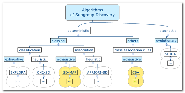
| 11 | Die
Analyse von Interaktionen im Data Mining |
Was sind Merkmals-Interaktionen?, CARs - Mining im Rahmen des Data Mining, Unterschiede zwischen und Gemeinsamkeiten von Associative Classification, Subgroup Discovery und Predictive Association Rules, Validierung eines Modells | speziell für Fortgeschrittene |
| 12 | Warum diese Seite? | "Standards" als Innovationshemmnis, Exkurs: Das Unbehagen an der klassischen Statistik, New Curriculum, New Statistics - There is life beyond 0.05, Kleiner Exkurs zu Kausalität und Korrelation, Erklärung und Beschreibung | |
| 13 | Plädoyer für eine "Konfigurations"-Statistik | Argumente für die Analyse von Merkmalsinteraktionen, Configurational Comparative Method, Treatment Heterogeneity, Realistic Evaluation, David Berliner und der "Schmetterlingseffekt" | |
| 14 | Links
und Quellenverzeichnis |
Basisliteratur zu Associative Classification, Subgroup Discovery und Supervised Association Rules, Literaturverzeichnis, Bilderverzeichnis | |
| 15 | Impressum | Impressum, Angaben zur Person, Kontaktdaten, Kontaktformular |
| 3. Illustrierendes Beispiel zum CARs - Mining |
| Geschlecht Alter Blutdruck Medikament |
| mann jung mittel drug_a |
| frau alt mittel drug_b |
| frau jung hoch drug_a |
| mann jung niedrig drug_b |
| frau alt hoch drug_a |
| mann jung mittel drug_a |
| frau alt mittel drug_b |
| mann jung niedrig drug_b |
| mann alt mittel drug_b |
| frau jung mittel drug_a |
| frau jung niedrig drug_b |
| mann alt hoch drug_a |
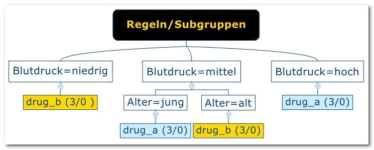
| IF Blutdruck=mittel
-> THEN drug= drug_a IF Blutdruck=niedrig -> THEN drug= drug_a IF Blutdruck=hoch -> THEN drug= drug_a IF Blutdruck=mittel, Alter=jung -> THEN drug= drug_a IF Blutdruck=mittel, Alter=alt -> THEN drug= drug_a ...usw. |
| Zielgrösse | ||||
| drug=drug_a | drug=Rest | |||
| Regel/Subgruppe | Blutdruck=mittel,
Alter=jung |
3 | 0 | 3 |
| Rest | 0 | 3 | 3 | |
| 3 | 3 | 6 (=n) |
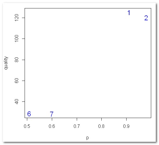
| Die
besten 10 Klassifikations-Regeln (= Subgruppen) für drug_a: nr quality p size description 1 1.5 1.00 3 Blutdruck=hoch 2 1.5 1.00 3 Blutdruck=mittel, Alter=jung 3 1.0 1.00 2 Geschlecht=mann, Blutdruck=mittel, Alter=jung 4 1.0 1.00 2 Blutdruck=hoch, Geschlecht=frau 5 1.0 1.00 2 Blutdruck=hoch, Alter=alt 6 0.5 1.00 1 Blutdruck=mittel, Alter=jung, Geschlecht=frau 7 0.5 1.00 1 Blutdruck=hoch, Geschlecht=mann 8 0.5 1.00 1 Blutdruck=hoch, Alter=jung 9 0.5 1.00 1 Blutdruck=hoch, Alter=alt, Geschlecht=frau 10 0.5 1.00 1 Blutdruck=hoch, Alter=jung, Geschlecht=frau |
| Die
besten 10 Klassifikations-Regeln (= Subgruppen) für drug_b: nr quality p size description 1 1.5 1.00 3 Blutdruck=niedrig 2 1.5 1.00 3 Alter=alt, Blutdruck=mittel 3 1.5 1.00 3 Blutdruck=niedrig, Alter=jung 4 1.0 1.00 2 Alter=alt, Blutdruck=mittel, Geschlecht=frau 5 1.0 1.00 2 Blutdruck=niedrig, Geschlecht=mann 6 1.0 1.00 2 Blutdruck=niedrig, Geschlecht=mann, Alter=jung 7 0.5 1.00 1 Alter=alt, Geschlecht=mann, Blutdruck=mittel 8 0.5 1.00 1 Blutdruck=niedrig, Geschlecht=frau 9 0.5 1.00 1 Blutdruck=niedrig, Geschlecht=frau, Alter=jung 10 0.5 0.60 5 Alter=alt |
| 4. Beispiel 2: Komplexe 3-Weg Interaktionen |
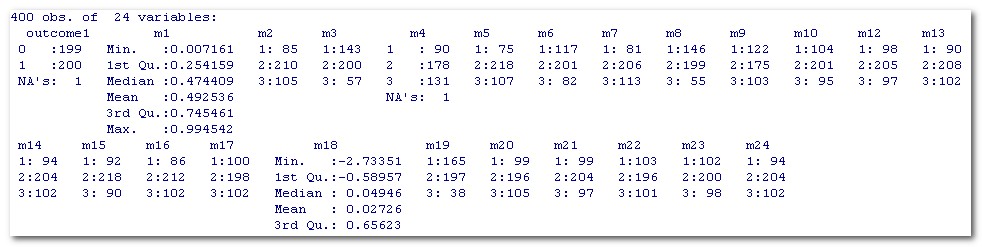 |
| m3 | m8 | m19 |
N outcome1 (1 / 0) |
hypergeometr.
Test p-Wert |
|
| Konfig. 1 | 1 | 1 | 3 | 12 / 1 | 0.003045509 |
| Konfig. 2 | 1 | 2 | 2 | 48 / 12 | 5.374803e-07 |
| Konfig. 3 | 1 | 3 | 1 | 22 / 2 | 2.272462e-05 |
| Konfig. 4 | 2 | 1 | 2 | 47 / 17 | 6.538334e-05 |
| Konfig. 5 | 2 | 2 | 1 | 47 / 14 | 6.101061e-06 |
| Konfig. 6 | 3 | 1 | 1 | 19 / 0 | 2.557732e-06 |
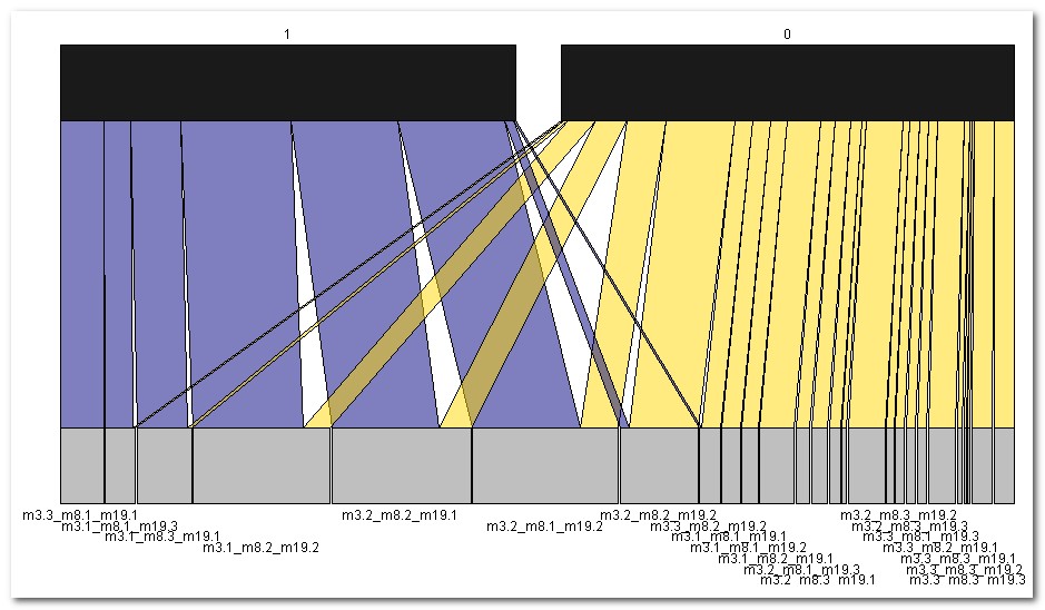
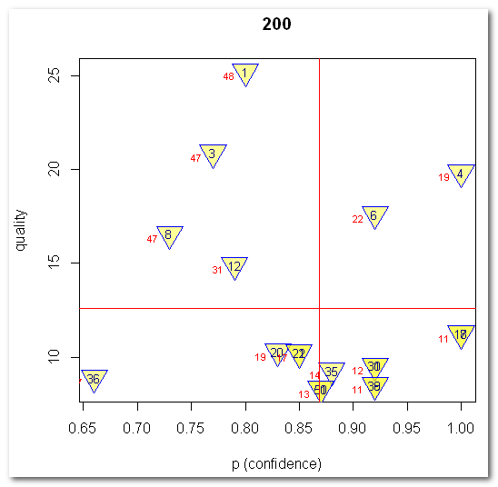
| Alle
bereinigten Klassifikations-Regeln (= Subgruppen) für outcome1=
1: nr chi2 p size description nZiel CohenW adj.RESIDUEN 1 25.21 0.80 60 m3=1, m19=2, m8=2 48 0.25 5.0 = Konfig.2 3 20.88 0.77 61 m19=1, m3=2, m8=2 47 0.23 4.6 = Konfig.5 4 19.85 1.00 19 m3=3, m8=1, m19=1 19 0.22 4.5 = Konfig.6 6 17.63 0.92 24 m8=3, m19=1, m3=1 22 0.21 4.2 = Konfig.3 8 16.57 0.73 64 m8=1, m19=2, m3=2 47 0.20 4.1 = Konfig.4 12 14.91 0.79 39 m6=3, m7=2 31 0.19 3.9 17 11.26 1.00 11 m8=3, m9=3, m19=1 11 0.17 3.4 18 11.26 1.00 11 m22=3, m7=3, m3=1 11 0.17 3.4 20 10.30 0.83 23 m9=3, m3=1, m7=2 19 0.16 3.2 21 10.24 0.85 20 m3=3, m6=2, m8=1 17 0.16 3.2 22 10.24 0.85 20 m4=1, m12=2, m19=1 17 0.16 3.2 30 9.56 0.92 13 m19=3, m3=1, m8=1 12 0.15 3.1 = Konfig.1 31 9.56 0.92 13 m6=3, m3=2, m10=2 12 0.15 3.1 35 9.31 0.88 16 m4=1, m5=3, m19=1 14 0.15 3.1 36 8.92 0.66 71 m3=1, m7=2 47 0.15 3.0 38 8.54 0.92 12 m10=3, m12=1, m15=2 11 0.15 2.9 39 8.54 0.92 12 m8=3, m9=3, m3=1 11 0.15 2.9 50 8.32 0.87 15 m4=1, m24=3, m19=1 13 0.14 2.9 51 8.32 0.87 15 m4=1, m14=3, m19=1 13 0.14 2.9 |
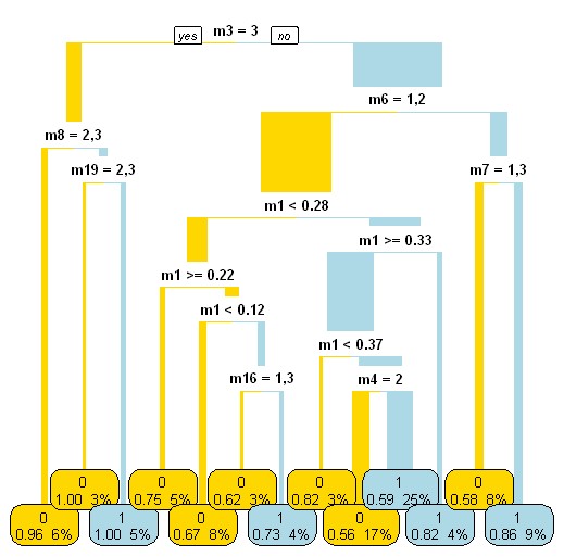 |
| Rule 14: (19, lift 1.9)
= Konfig. 6 m3 = 3 m8 = 1 m19 = 1 -> outcome1=1 [0.952] Rule 15: (61/14, lift 1.5) = Konfig. 5 m3 = 2 m8 = 2 m19 = 1 -> outcome1=1 [0.762] Rule 16: (64/17, lift 1.5) = Konfig. 4 m3 = 2 m8 = 1 m19 = 2 -> outcome1=1 [0.727] Rule 17: (143/61, lift 1.1) m3 = 1 -> outcome1=1 [0.572] |
| Number
of Rules : 3 (m1 <= 0.237832) => outcome1=0 (96.0/39.0) (m19 = 3) => outcome1=0 (31.0/9.0) Rest => outcome1=1 (272.0/120.0) |
| 5. Beispiel 3: Haupteffekte reichen aus |
| 150
obs. of 5 variables: Sepal.Length Sepal.Width Petal.Length Petal.Width Species Min. :4.300 Min. :2.000 Min. :1.000 Min. :0.100 setosa :50 1st Qu.:5.100 1st Qu.:2.800 1st Qu.:1.600 1st Qu.:0.300 versicolor:50 Median :5.800 Median :3.000 Median :4.350 Median :1.300 virginica :50 Mean :5.843 Mean :3.057 Mean :3.758 Mean :1.199 3rd Qu.:6.400 3rd Qu.:3.300 3rd Qu.:5.100 3rd Qu.:1.800 Max. :7.900 Max. :4.400 Max. :6.900 Max. :2.500 |
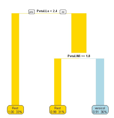 |
| Rule: (Petal.Length >= 2.4) and (Petal.Width < 1.8) => outcome1=versicolor (.91/ 36%) === Confusion Matrix === a b <-- classified as 95 1 | a = Rest 5 49 | b = versicolor Kappa statistic = .91 |
Rule 4: (48/1, lift 2.9) Petal.Length > 1.9 Petal.Length <= 4.9 Petal.Width <= 1.7 -> outcome1= versicolor [0.960] |
| Evaluation
on training data (150 cases): Rules ---------------- No Errors 4 4( 2.7%) === Confusion Matrix === (a) (b) <-classified as ---- ---- 99 1 (a): class Rest 3 47 (b): class versicolor Kappa statistic = .94 |
Number of Rules : 2 (Petal.Length >= 3.5) and (Petal.Width <= 1.6) and (Petal.Length <= 4.9) => outcome1=versicolor (44.0/0.0) => outcome1=Rest (106.0/6.0) |
| === Summary === Correctly Classified Instances 144 96 % Incorrectly Classified Instances 6 4 % Kappa statistic 0.9072 Mean absolute error 0.0755 Root mean squared error 0.1943 Relative absolute error 16.9532 % Root relative squared error 41.2077 % Coverage of cases (0.95 level) 100 % Mean rel. region size (0.95 level) 85.3333 % Total Number of Instances 150 === Confusion Matrix === a b <-- classified as 100 0 | a = Rest 6 44 | b = versicolor |
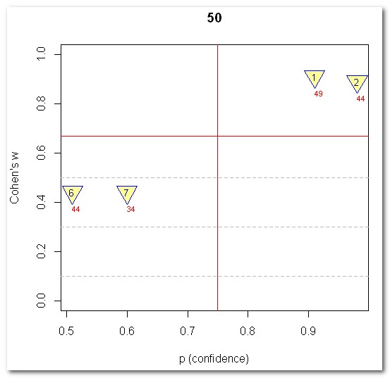
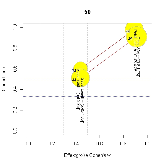
| Alle
bereinigten Klassifikations-Regeln (= Subgruppen) für Species=
versicolor: nr chi^2 p size description nz1 CohenW adj.RESIDUEN Errors Kappa 1 125.13 0.91 54 Petal.Width='(0.8-1.75]' 49 0.91 11.2 6 .91 2 120.14 0.98 45 Petal.Length='(2.45-4.75]' 44 0.89 11.0 7 .89 6 28.83 0.51 86 Sepal.Length='(5.45-7.05]' 44 0.44 5.4 50 .39 7 28.65 0.60 57 Sepal.Width='(-inf-2.95]' 34 0.44 5.4 39 .43 Zum Vergleich: aussortierte, zu Regel 2 redundante Regel 3 3 120.14 0.98 45 Petal.Length='(2.45-4.75]' 44 0.89 11.0 7 .89 + Petal.Width='(0.8-1.75]' |
| === Confusion Matrix zu Regel
1 === (a) (b) <-classified as ---- ---- 95 5 (a): class Rest 1 49 (b): class versicolor Kappa statistic = .91 |
| Logistische Regression: | Lineare Diskriminanzanalyse: |
| Anova(GLM,
type="II", test="LR") Analysis of Deviance Table (Type II tests) Response: outcome1 LR Chisq Df Pr(>Chisq) Sepal.Length 0.1431 1 0.70524 Sepal.Width 15.6969 1 7.434e-05 *** Petal.Length 3.9518 1 0.04682 * Petal.Width 6.4089 1 0.01135 * |
Coefficients
of linear discriminants: LD1 Sepal.Length -0.0966345 Sepal.Width -2.1366766 Petal.Length 1.0580824 Petal.Width -2.3701409 |
| ===
Confusion Matrix === a b <-- classified as 86 25 | a = Rest 14 25 | b = versicolor Errors = 39 Kappa statistic = .38 |
===
Confusion Matrix === a b <-- classified as 86 26 | a = Rest 14 24 | b = versicolor Errors = 40 Kappa statistic = .36 |
| 6.
Hinweise und Tipps zur Durchführung des CARs - Mining |
 |
 |
 |
 |
| Zielgrösse | ||||
| von Interesse | Rest | |||
| Regel/Subgruppe | von Interesse | a | b | a+b |
| Rest | c | d | c+d | |
| a+c | b+d | n |
 |
| Alle
bereinigten Klassifikations-Regeln (= Subgruppen) für Species=
versicolor: nr quality p size description nZiel CohenW adj.RESIDUEN Errors Kappa 1 125.13 0.91 54 Petal.Width='(0.8-1.75]' 49 0.91 11.2 6 .91 2 120.14 0.98 45 Petal.Length='(2.45-4.75]' 44 0.89 11.0 7 .89 6 28.83 0.51 86 Sepal.Length='(5.45-7.05]' 44 0.44 5.4 50 .39 7 28.65 0.60 57 Sepal.Width='(-inf-2.95]' 34 0.44 5.4 39 .43 |
 |
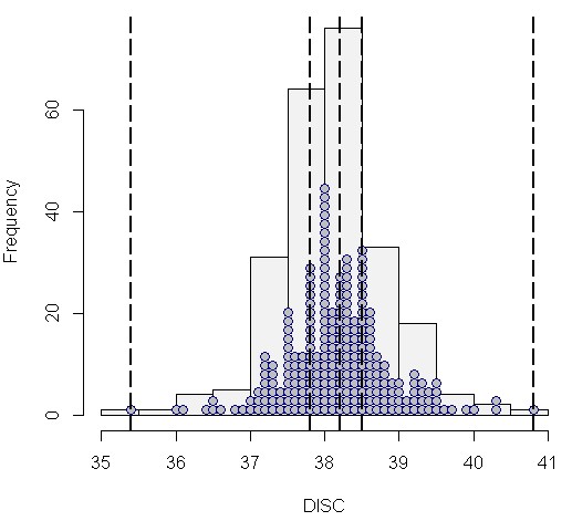
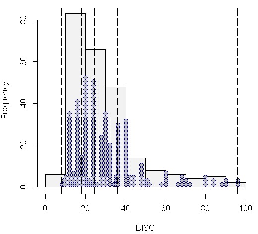
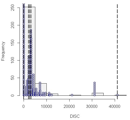
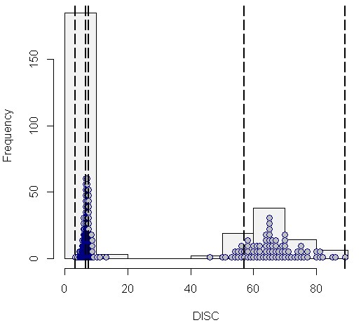
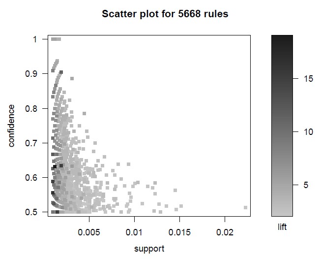
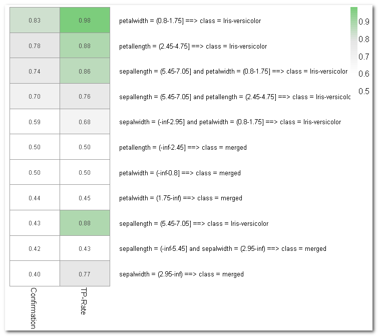
Auf diese Weise sind die wichtigsten Ergebnisse der erweiterten Ausgabedatei in einem Streudiagramm übersichtlich zusammen gefasst. So lassen sich leicht die zentralen Regeln/Subgruppen erkennen: Solche mit hoher Effektgröße und idealerweise gleichzeitig möglichst hoher Confidence und Fallzahl. Die (heurostatistische) Signifikanz der interessantesten Regeln/Subgruppen lässt sich dann aus der Ergebnisdatei ablesen.
Als letzte Form der Visualisierung ist mit Plot 4 eine so genannte Heatmap empfehlenswert. So kann man die interessanten Regeln/Subgruppen leicht anhand ihrer Färbung identifizieren: je grüner desto interessanter. Zu diesem Zweck werden die Kennwerte der Ausgabedatei (hier quality, p, nZiel) spaltenweise standardisiert, mit einem Mittelwert von jeweils 0. Je mehr eine Regel/Subgruppe positiv von der durchschnittlichen Verteilung aller Regeln abweicht, umso grüner (und interessanter) ist sie.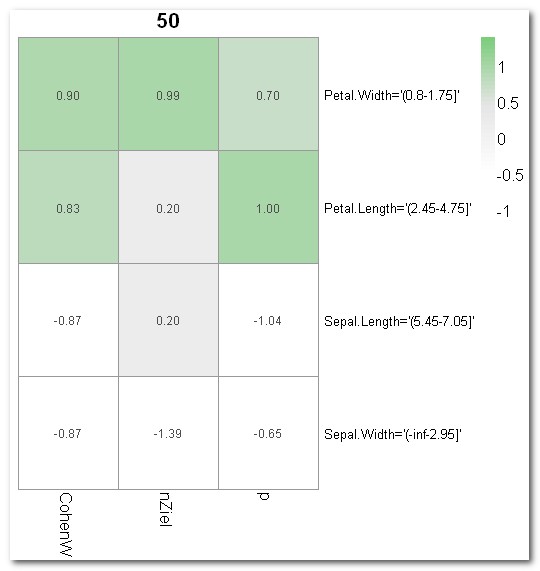
|
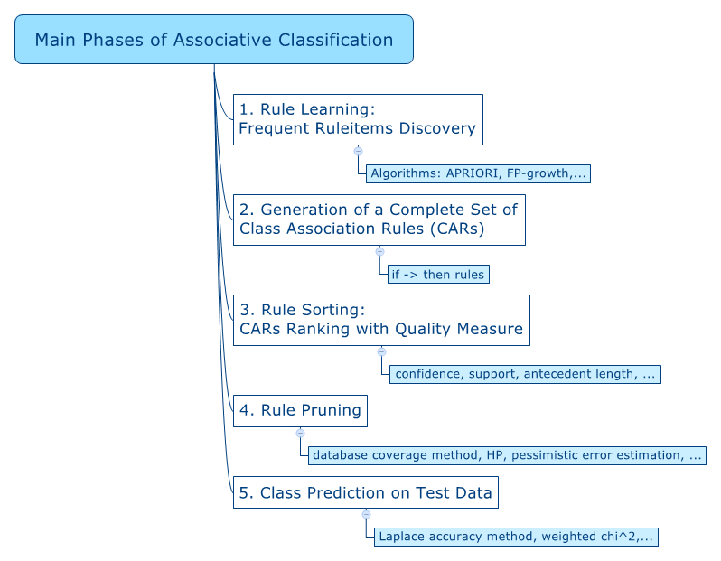
| 7. Freeware zum CARs - Mining |
| Software | CARs-Klasse | Algorithmen | Besonderheiten | "Association Mining-Paradigma" | Link |
| Stand alone Programme | |||||
| Cortana | Subgroup Discovery | Beam-Search u.a. | ohne Pruning | nein | http://datamining.liacs.nl/cortana.html |
| Vikamine | Subgroup Discovery | SD-Map, Beam-Search, BSD | - | u.a. | http://www.vikamine.org |
| Data Mining Suiten | |||||
| Keel | Associative
Classification, Subgroup Discovery |
Associative
Classification: CBA, CBA2, CPAR, CMAR, FCRA, CFAR, FARC-HD Subgroup Discovery: CN2-SD, Apriori-SD, SD-Algorithm, SDIGA, NMEEF, MESDIF, SD-Map |
sämtliche neueren Ansätze zur Knowledge Discovery (spez. Evolutionary Algorithms) | u.a. | http://www.keel.es |
| Knime | Subgroup Discovery | Beam-Search | Plug in "Cortana" (s.o.), ohne Pruning | nein | https://www.knime.org/ |
| Orange | Subgroup Discovery | SD, CN2-SD, Apriori-SD | Toolkit "Subgroup Discovery" | nein | http://orange.biolab.si/ |
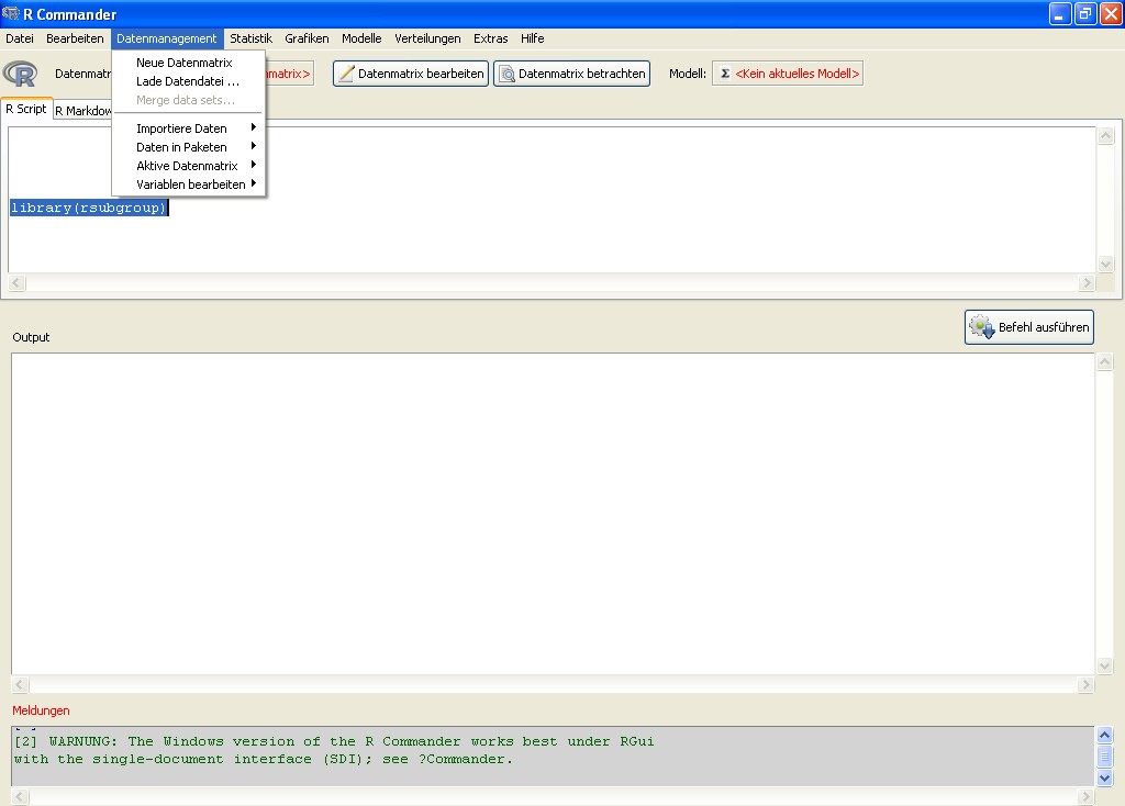
| R-Project | Subgroup Discovery | SD-Map, Beam-Search, BSD | package (rsubgroup); entspricht "Vikamine" (s.o.) | u.a. | http://www.r-project.org/ |
| Rapid Miner | Subgroup Discovery | SD, CN2-SD | Extension "Subgroup Discovery" | nein | https://rapidminer.com/ |
| Tanagra | supervised/ predictive Association Rules | supervised APRIORI | ASSOC SPV, SPV RULE TREE ASSOC | ja | http://eric.univ-lyon2.fr/ ~ricco/tanagra/en/tanagra.html |
| Weka | Associative Classification, supervised/ predictive Association Rules | JCBA, Predictive Apriori, Tertius | gleichnamige
CAR-Classifiers- und Association-packages |
ja | http://www.cs.waikato.ac.nz/ml/weka/ |
| 8.
Kleine Einführung in die
Nutzung der Software R-Project von CRAN |
 |
 |
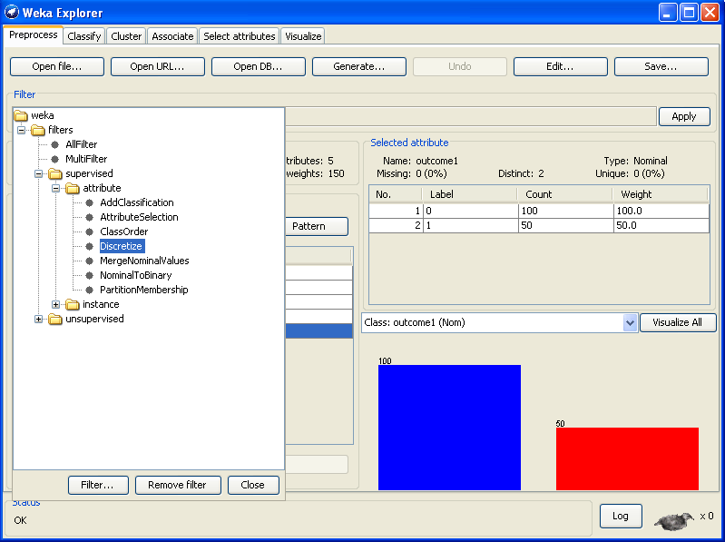
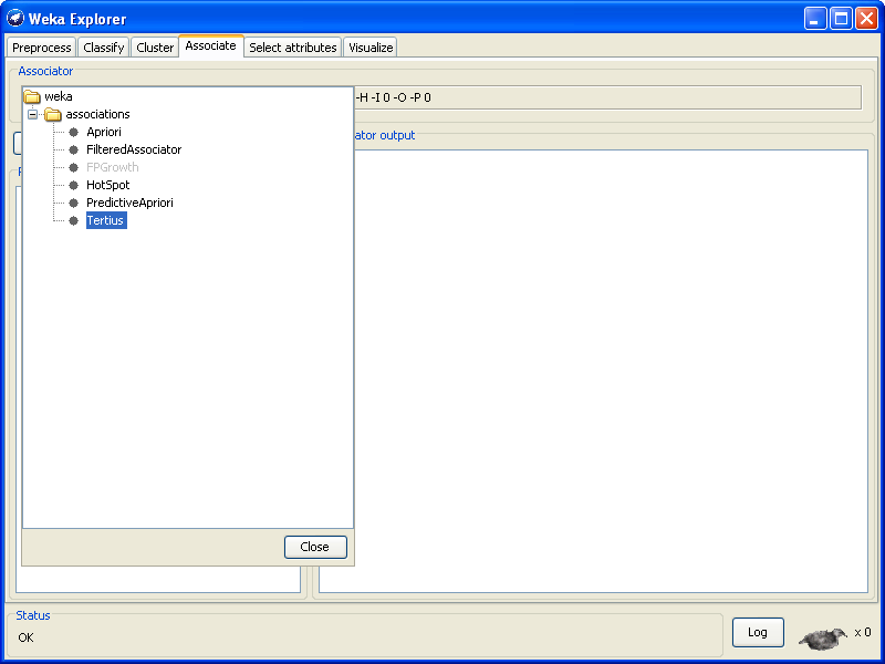
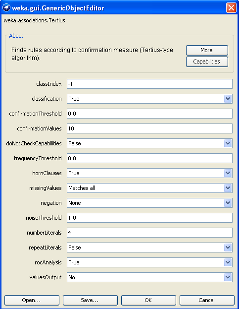
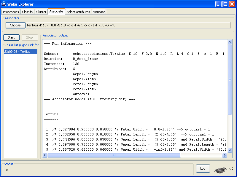
| 9. CARs - Mining mit WEKA TERTIUS |

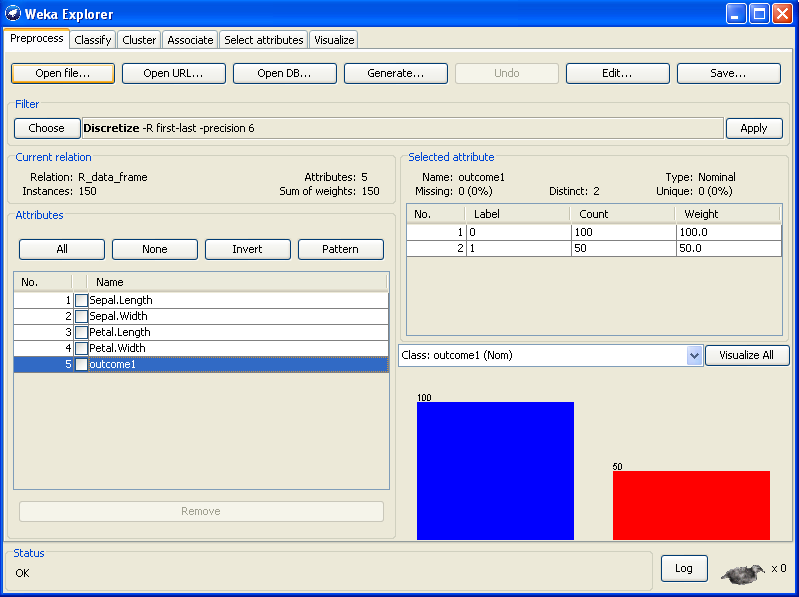
| @RELATION
iris @ATTRIBUTE sepallength REAL @ATTRIBUTE sepalwidth REAL @ATTRIBUTE petallength REAL @ATTRIBUTE petalwidth REAL @ATTRIBUTE class {Iris-setosa,Iris-versicolor,Iris-virginica} @DATA 5.1,3.5,1.4,0.2,Iris-setosa 4.9,3.0,1.4,0.2,Iris-setosa 4.7,3.2,1.3,0.2,Iris-setosa 4.6,3.1,1.5,0.2,Iris-setosa 5.0,3.6,1.4,0.2,Iris-setosa 5.4,3.9,1.7,0.4,Iris-setosa ... |
| 10. Zum
Verhältnis
von klassischer Statistik und Data Mining |
| Bereich | Klassischer statistischer Ansatz | Data
Mining im Rahmen des Knowledge Discovery |
| Kurzcharakterisierung |  |
 |
| Definition | "Statistics,
especially as taught in most
statistics texts, might be described as being characterized by
data sets which are small and clean, which permit straightforward
answers via intensive analysis of single data sets, which are static,
which were sampled in an iid manner, which were often collected to
answer the particular problem being addressed, and which are solely
numeric." (Hand 1998) |
"Data
mining is the nontrivial process of
identifying valid, novel, potentially useful, and ultimately
understandable patterns in data." (Fayyad 1996) |
| Paradigma | deduktiv weil i.d.R. Theorie-basiert, induktiv bei Inferenzschlüssen | induktiv weil heuristisch |
| Art der Analyse | konfirmativ:
Hypothesen testend, auf Population bezogen - "Testing hypothesis" |
explorativ:
Muster entdeckend, auf Datensatz beschränkt - "Finding the right hypothesis" |
| Datengewinnung | erst auf der Basis des Forschungsdesigns | Daten liegen i.d.R. schon vor, Sekundäranalyse |
| Fallzahlen | eher klein | eher groß |
| Variablenumfang | klein | sehr groß |
| Datenqualität | i.d.R. hoch | "dirty", mit fehlenden Werten |
| Skala der Merkmale | überwiegend metrisch | gemischtes Skalenniveau |
| dominierende Modellklasse | Regression (metrische Zielgröße) | Klassifikation (kategoriale Zielgröße) |
| Analyse-Philosophie | "The model is king":
voraussetzungsvolle mathematische und inhaltliche, theoretische Modelle. Die Daten müssen den Anwendungsvoraussetzungen der mathematischen Modelle entsprechen. |
"The data is king":
möglichst modellarm ("nah an den Daten") und voraussetzungsfrei. Die Verfahren sollen den Daten "folgen" und nicht die Daten dem mathematischen Modell. |
| Durchführung | Standardisiertes "Kunsthandwerk" | Weitgehend automatisiert |
| Modellvoraussetzungen | In der Praxis (sozialwissenschaftlicher Forschung) häufig unrealistisch: multivariate Normalverteilung, unkorrelierte Prädiktoren, Varianzhomogenität, keine Ausreißer, keine fehlenden Werte, Zusammenhänge der Merkmale sind lediglich linear und additiv, theoretische Prüfverteilungen anstatt empirischer, ... | I.d.R.
gering. Gemischte Skalenniveaus, fehlende Werte
und Interkorrelationen können problemlos verarbeitet werden
(z.B. bei
Entscheidungsbäumen). Bei einigen Verfahren (z.B. Associative Classification) wird aber ein kategoriales Skalenniveau aller Merkmale verlangt (ggf. "supervised discretization" nötig). |
| Umgang mit Merkmalsinteraktionen | Interaktionen widersprechen i.d.R. den Modellvoraussetzungen und müssen zudem expizit und ex ante definiert werden. Deren Berücksichtigung führt gleichwohl zu instabilen Schätzern (Multikollinearität). | Gerade auch Interaktionen höherer Ordnung (z.B. 3-Weg- oder 4-Weg-Interaktionen) stehen i.d.R. im Fokus der Analyse, werden exploriert. |
| Erkenntnisgewinn | "Auspartialisierte
Effekte", d.h.: von den Wirkungen der anderen
erklärenden Variablen bereinigte Effekte der einzelnen
Merkmale; oder
anders formuliert: Die Erklärungskraft einer Variablen, wenn
die Wirkung aller
anderen Variablen "herausgerechnet" ist. Bei dieser Art von "1-Variablen-Statistik" bleibt das Zusammenwirken der Merkmale unterbelichtet. |
Merkmalsinteraktionen, Merkmalskonfigurationen, Moderatoren, Resilienzfaktoren, homogene Subgruppen, homogene Segmente oder nicht-lineare Zusammenhänge werden identifiziert. |
| Gesellschaftlicher Anwendungsbereich | Wissenschaft, akademischer Bereich | Ursprünglich überwiegend Business-Bereich. Zunehmend auch Bereiche der wiss. Forschung mit Massendaten wie z.B. Astronomie, Meteorologie, Gesundheitswissenschaften, Bioinformatik, speziell Genomforschung, etc. |
| Software-Implementierung | Ursprünglich überwiegend kommerziell | Kommerziell und Freeware-Tools der Machine Learning- und Data Mining-Community |
| Typische Verfahren | Linear Regression, ANOVA, MANOVA, Discriminant Analysis, Logistic Regression, GLM, Factor Analysis, ... | Decision Tree Induction, Rule Induction, Association Rules, Associative Classification, Subgroup Discovery, Nearest Neighbors, Clustering Methods, Feature Extraction, Visualization, Neural Networks, Genetic Algorithms, Self-Organizing Maps, ... |
| Hardware-Voraussetzungen | Gering, wg. restriktiver Annahmen der statistischen, mathematischen Modelle (theoretische Prüfverteilungen, lineare Statistik, ...) | Eher hoch, wegen geringer Restriktionen der Modelle (Verfahren "folgen" den Daten und nicht die Daten dem mathematischen Modell). Bei einigen Verfahren Implementierung von Parallel-Computing sinnvoll. |
| 11. Die Analyse von
Interaktionen im Data Mining |
 |
 |
| 12. Warum diese Seite? |
 |
 Und weil
den
Und weil
den  Statistikern von
damals
(die häufig Mathematiker waren)
kein Computer zur Verfügung stand - mit dem sie zum
Beispiel
das konzeptionell einfache aber rechenintensive
Randomization Model statistischer Inferenz von
Fisher
1936 hätten umsetzen können -,
waren sie gezwungen, rigide und voraussetzungsvolle, häufig
datenferne mathematische Modelle zu entwerfen, die sie
überhaupt
erst in die Lage versetzten, größere Datenmengen zu
verarbeiten. Doch dadurch wurden die Statistiker
von ihren Mitmenschen nicht mehr verstanden, was bis heute ihr
Herrschaftswissen und das häufige Unbehangen
gegenüber dieser
Disziplin bei vielen Studenten/innen begründet. Und mit
rudimentären Kenntnissen dieser "Steinzeit"-Statistik
ausgestattet, führen jedes Jahr Zehntausende von
Studenten/innen der Soziologie, Erziehungswissenschaft, Sozialen
Arbeit, Politologie etc. ihre
empirischen Forschungsarbeiten durch, produzieren dabei mitunter meh
Statistikern von
damals
(die häufig Mathematiker waren)
kein Computer zur Verfügung stand - mit dem sie zum
Beispiel
das konzeptionell einfache aber rechenintensive
Randomization Model statistischer Inferenz von
Fisher
1936 hätten umsetzen können -,
waren sie gezwungen, rigide und voraussetzungsvolle, häufig
datenferne mathematische Modelle zu entwerfen, die sie
überhaupt
erst in die Lage versetzten, größere Datenmengen zu
verarbeiten. Doch dadurch wurden die Statistiker
von ihren Mitmenschen nicht mehr verstanden, was bis heute ihr
Herrschaftswissen und das häufige Unbehangen
gegenüber dieser
Disziplin bei vielen Studenten/innen begründet. Und mit
rudimentären Kenntnissen dieser "Steinzeit"-Statistik
ausgestattet, führen jedes Jahr Zehntausende von
Studenten/innen der Soziologie, Erziehungswissenschaft, Sozialen
Arbeit, Politologie etc. ihre
empirischen Forschungsarbeiten durch, produzieren dabei mitunter meh r
Methodenartefakte als substanziellen wissenschaftlichen Zugewinn - weil
sie die benutzten statistischen Modelle nicht wirklich verstehen -
und werden anschließend auf
die Berufswelt losgelassen, in der ihnen diese Art von Statistik i.d.R.
wenig hilfreich ist.
r
Methodenartefakte als substanziellen wissenschaftlichen Zugewinn - weil
sie die benutzten statistischen Modelle nicht wirklich verstehen -
und werden anschließend auf
die Berufswelt losgelassen, in der ihnen diese Art von Statistik i.d.R.
wenig hilfreich ist. 
 ng von Standards
bedeutet
faktisch die Behinderung des wissenschaftlichen Fortschritts. Denn wer
den Modestandard nicht hält, der bekommt seine Artikel nicht
in
Review-Zeitschriften unter und dessen Karrierechancen sinken rapide.
Standards zementieren den aktuellen Stand der Unwissenheit.
Und
Standards sind ziemlich hartnäckig.
ng von Standards
bedeutet
faktisch die Behinderung des wissenschaftlichen Fortschritts. Denn wer
den Modestandard nicht hält, der bekommt seine Artikel nicht
in
Review-Zeitschriften unter und dessen Karrierechancen sinken rapide.
Standards zementieren den aktuellen Stand der Unwissenheit.
Und
Standards sind ziemlich hartnäckig.  rtschritt
nicht als ein kontinuierlicher, kumulativer Prozess des Zugewinns an
Erkenntnis vollzieht sondern als ein eruptiver, revolutionärer
Paradigmenwechsel nach dem Motto "Alles wieder zurück
auf
Start" (vgl. den Inkommensurabilitätsbegriff von Kuhn (1962)
und
Feyerabend (1976, 1978)).
rtschritt
nicht als ein kontinuierlicher, kumulativer Prozess des Zugewinns an
Erkenntnis vollzieht sondern als ein eruptiver, revolutionärer
Paradigmenwechsel nach dem Motto "Alles wieder zurück
auf
Start" (vgl. den Inkommensurabilitätsbegriff von Kuhn (1962)
und
Feyerabend (1976, 1978)). | "Randomized
rather than random-sampling designs are used in most
comparative biomedical experiments. On the basis of pure theory,
statistical inferences from the experiments are valid only under the
randomization model of inference. Why, then, do biomedical
investigators not employ exact or sampled permutation tests to
analyze their results? A trivial reason is that editors of biomedical journals might not understand permutation tests and their statistical advisers might not accept the arguments we have put forward. Our personal experience is that it is much easier to get a manuscript published if one stays with classical tests under the population model. There is also an important practical point. There are plenty of microcomputer statistical software packages with which to perform classical or modified t and F tests, but a dearth of software for performing permutation tests for differences between means." (ebd. 131) |
| "For
more than 50 years,
however, leading scholars — Paul Meehl, Jacob Cohen, and many
others — have
explained the deep flaws of NHST and described how it damages research
progress. ... Statistics teaching, textbooks, software, the APA Publication Manual, journal guidelines, and universal practice all largely centered on NHST. We claimed to be a science, but could not change our methods in the face of evidence and cogent argument that there are vastly better ways. ...In 2005, Stanford University Professor of Medicine John Ioannidis connected the dots in a famous article titled “Why Most Published Research Findings Are False.” He identified the overwhelming imperative to achieve statistical significance as a core problem. It was imperative because it was the key to publication, and thus to jobs and funding. ... Most excitingly, NHST was, at long last, subjected to renewed scrutiny. The 2010 edition of the APA Publication Manual included the unequivocal statement that researchers should “wherever possible, base discussion and interpretation of results on point and interval estimates.” It included for the first time numerous guidelines for reporting CIs." (Cumming 2014b) |
| Exegese
über das Anbinden von Katzen während des
Gottesdienstes Jeden Abend hielt Bruder Michael eine Andacht, und immer störte ihn dabei eine Katze. Der Bruder bat deshalb, die Katze während des Gottesdienstes anzubinden. Als Bruder Michael gestorben war, band man die Katze weiterhin an. Als diese Katze starb, fand man eine andere, die man während des Gottesdienstes anbinden konnte. Drei Jahrhunderte später begannen die theologischen Gelehrten, Abhandlungen über das Mysterium des Anbindens von Katzen während des Gottesdienstes zu verfassen. Das Problem ist noch immer nicht gelöst. (Marco Aldinger nach Joachim-Ernst Behrendt 1996, 80) |
| EXKURS: Das Unbehagen an der klassischen Statistik |
 satisfied in practice ... The model must follow the data. and not the
other way around. This is another error in the application of
mathematics to the human sciences: the abundance of models, which are bu
satisfied in practice ... The model must follow the data. and not the
other way around. This is another error in the application of
mathematics to the human sciences: the abundance of models, which are bu ilt
a priori and then confronted with the data by what one calls a 'test'.
Often the 'test' is used to justify a model in which the number of
parameters to be fitted is larger than the number of data points."
(Benzecri 1973, nach Gifi 1990, 25)
ilt
a priori and then confronted with the data by what one calls a 'test'.
Often the 'test' is used to justify a model in which the number of
parameters to be fitted is larger than the number of data points."
(Benzecri 1973, nach Gifi 1990, 25) ple discrete models
perhaps,
such models are never
exactly true". (Hampel 1973, 87f)
ple discrete models
perhaps,
such models are never
exactly true". (Hampel 1973, 87f)
|
"In the 1950s, psychology
started adopting null-hypothesis
significance testing (NHST), probably because
it seemed to offer a scientific, objective way to draw conclusions from
data.
NHST caught on in a big way and now almost all empirical research is
guided by p
values — which are in fact tricky conditional probabilities
that few understand
correctly. Why did NHST become so
deeply entrenched? I suspect it’s the seductive but
misleading hints of
importance and certainty — even truth — in a
statement that we’ve found a
“statistically significant effect.” NHST decisions can be
wrong, and every
decent textbook warns that a statistically significant effect may be
tiny and
trivial. But we so yearn for certainty that we take statistical
significance as
pretty close. ... In 1990 Rothman founded the journal Epidemiology, stating that it would not publish NHST. For the decade of his editorship, it flourished and published no p values, demonstrating that successful science does not require NHST. In psychology, APS Fellow Geoff Loftus edited Memory & Cognition from 1993 to 1997 and strongly encouraged figures with error bars — such as CIs — instead of NHST. He achieved some success, but subsequent editors returned to NHST business as usual. ... Then came reports that some
well-accepted results could not be replicated. From cancer research to
social
psychology, it seemed that an unknown proportion of results published
in good
journals were simply incorrect. This was devastating — which
scientific results
could we trust? Ioannidis argued
convincingly that the combination of these three effects of reliance on
NHST
may indeed have resulted in most published findings being false.
Suddenly this
was serious — the foundations of our science were creaking.
Happily, a range of
imaginative responses have now emerged and are developing fast
— several are
described elsewhere in this issue of the Observer. Most excitingly, NHST was, at long last, subjected to renewed scrutiny. The 2010 edition of the APA Publication Manual included the unequivocal statement that researchers should “wherever possible, base discussion and interpretation of results on point and interval estimates.” It included for the first time numerous guidelines for reporting CIs." |
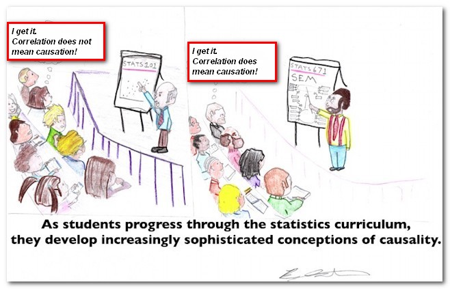
| Kleiner
Exkurs zu Kausalität und Korrelation, Erklärung und Beschreibung |
 nstrukt.
Und Kausalität ist vor allem ein menschliches
Bedürfnis. Kein
Mensch weiß, ob es Kausalität wirklich gibt und wenn
ja, in welcher Form. Im Verständnis eines Radikalen
Konstruktivismus ist "Kausalität" aber mitunter eine ganz nützliches
Konstrukt - um beispielsweise tragfähige Brücken zu
bauen - aber sie
ist deshalb bei weitem noch keine wirkliche, wahre Entität.
Kausalität
entsteht - als gutes Kino - erst im Kopf des Betrachters.
nstrukt.
Und Kausalität ist vor allem ein menschliches
Bedürfnis. Kein
Mensch weiß, ob es Kausalität wirklich gibt und wenn
ja, in welcher Form. Im Verständnis eines Radikalen
Konstruktivismus ist "Kausalität" aber mitunter eine ganz nützliches
Konstrukt - um beispielsweise tragfähige Brücken zu
bauen - aber sie
ist deshalb bei weitem noch keine wirkliche, wahre Entität.
Kausalität
entsteht - als gutes Kino - erst im Kopf des Betrachters.  liens beispielsweise sind
unterschiedliche
Zeitdimensionen in nicht-linearer Form miteinander
verschränkt.Wie
gesagt: Kausalität entsteht - als gutes Kino - erst im Kopf
des
Betrachters.
liens beispielsweise sind
unterschiedliche
Zeitdimensionen in nicht-linearer Form miteinander
verschränkt.Wie
gesagt: Kausalität entsteht - als gutes Kino - erst im Kopf
des
Betrachters. | 13. Plädoyer
für eine "Konfigurations-Statistik" - für Analysen mit dem Fokus auf Merkmalsinteraktionen |
Die QCA bildet das auswertungstechnische Pendant für die von Fend (2004) im erziehungswissenschaftlichen Kontext (der internationalen Schülerleistungsvergleiche, PISA etc.) formulierte Forschungsperspektive, anstatt auf einzelne erklärende Variablen besser auf Konfigurationen von Merkmalen erfolgreicher Länder zu fokussieren. Denn es gelte zu berücksichtigen, dass hohe durchschnittliche Schülerleistungen mit unterschiedlichen, funktional äquivalenten Konfigurationen möglich sind, da die einzelnen Merkmale in verschiedenen Ländern ganz unterschiedliche Bedeutungen besitzen können und Bestandteil eines komplexen länderspezifischen Kontextes von Bedingungsvariablen sind, der die Wirkung dieser Merkmale verstärken oder kompensieren könne. Das Schweizerische Bundesamt für Statistik (Holzer 2005) hat genau vor diesem konzeptionellen Hintergrund mittels QCA eine instruktive Modellierung der differentiellen Einflussfaktoren der Schülerleistungen für die Schweizer Kantone anhand einer Reanalyse der PISA 2003-Daten vorgelegt.
Unabhängig davon, wie man im Detail zum technischen Ansatz der QCA steht (siehe auch meine Kritik oben):| "When
two alternative treatments (A and B) are available, some subgroup
of patients may display a better outcome with treatment A than with B,
whereas for another subgroup, the reverse may be true. If this is the
case, a qualitative (i.e., disordinal) treatment–subgroup
interaction
is present. Such interactions imply that some subgroups of patients
should be treated differently and are therefore most relevant for
personalized medicine. ... In the presence of a qualitative treatment–subgroup interaction, the question ‘Which treatment is better, A or B?’ becomes meaningless and should be replaced by ‘Which treatment is best for which kind of patients?’. The moderator variable(s) contributing to the qualitative interaction(s) then identify for whom and under which circumstances treatment A is better than B and for whom the reverse is true. As such, they represent important patient characteristics that may be used in the future to set up an optimal treatment assignment strategy to support healthcare decision makers. It is, therefore, essential to uncover qualitative treatment–subgroup interactions with an appropriate statistical method." (Dusseldorp, Van Mechelen 2014, 219-220) |
"... In my estimation, we have the hardest-to-do science of them all! We do our science under conditions that physical scientists find intolerable. We face particular problems and must deal with local conditions that limit generalizations and theory building—problems that are different from those faced by the easier-to-do sciences. ... In education, broad theories and ecological generalizations often fail because they cannot incorporate the enormous number or determine the power of the contexts within which human beings find themselves. ... It was found that the variance in student achievement was larger within programs than it was between programs. No program could produce consistency of effects across sites. Each local context was different, requiring differences in programs, personnel, teaching methods, budgets, leadership, and kinds of community support. These huge context effects cause scientists great trouble in trying to understand school life. ... Doing science and implementing scientific findings are so difficult in education because humans in schools are embedded in complex and changing networks of social interaction. The participants in those networks have variable power to affect each other from day to day, and the ordinary events of life (a sick child, a messy divorce, a passionate love affair, migraine headaches, hot flashes, a birthday party, alcohol abuse, a new principal, a new child in the classroom, rain that keeps the children from a recess outside the school building) all affect doing science in school settings by limiting the generalizability of educational research findings. Compared to designing bridges and circuits or splitting either atoms or genes, the science to help change schools and classrooms is harder to do because context cannot be controlled. ... Context is of such importance in educational research because of the interactions that abound. The study of classroom teaching, for example, is always about understanding the 10th or 15th order interactions that occur in classrooms. Any teaching behavior interacts with a number of student characteristics, including IQ, socioeconomic status, motivation to learn, and a host of other factors. Simultaneously, student behavior is interacting with teacher characteristics, such as the teacher’s training in the subject taught, conceptions of learning, beliefs about assessment, and even the teacher’s personal happiness with life. But it doesn’t end there because other variables interact with those just mentioned—the curriculum materials, the socioeconomic status of the community, peer effects in the school, youth employment in the area, and so forth. Moreover, we are not even sure in which directions the influences work, and many surely are reciprocal. Because of the myriad interactions, doing educational science seems very difficult, while science in other fields seems easier." (Berliner 2002,18-20) |
| 14. Links und Quellenverzeichnis |
| 15. Impressum |